How much should I save for retirement?
Most people ask themselves this question at some point in their working life (hopefully, relatively early). With the continued shift toward defined contribution plans, future retirees are being asked to take on more responsibility for their retirement outcomes than in the past. So the question is of vital importance. But do we have a good answer?
First, it is important to note that simple rules of thumb do not work for many people. When planning for retirement, income uncertainty can be substantial, so a one-size-fits-all solution is unlikely to work. In particular, the saving rate that works well on average does not work well for people with steep income trajectories or high-income variation over their working life—the very people who may need to rely more on personal savings.
We have found that what works is a tailored solution that incorporates the characteristics of each household. Specifically, dynamic approaches that take more information into account will improve retiree success rates. One crucial piece of information is household income. We derive income-based saving rates that work across many income profiles, particularly for high-income, high-variability individuals. As income changes over time, individuals increase their saving rates as income grows, with downward adjustments if income declines. Following this rule, different individuals at different stages of their careers (or different income levels) will have different saving rates.
Saving rates that depend on income levels make sense: Households with high income during their working years have more income that needs to be replaced during retirement. The willingness and ability to save also tend to rise with income. A dynamic approach to saving accommodates changing retirement needs and savings capacity.
Our simulations account for uncertainty in both income and investment returns. We simulate potential career paths for 100,000 households using data from the PSID, the largest longitudinal dataset on income and other demographics in the world.1 Savings are invested in a mix of Treasury bonds and global equities, following three alternative allocation strategies. Equity and bond returns are bootstrapped using historical data.
We use our simulations to study the impact of income, saving rates, and age on retirement outcomes. Throughout the paper, we define successful outcomes as achieving a targeted replacement rate with a high degree of confidence. We find that saving consistently and throughout one’s career is crucial to a successful retirement. Increasing the probability of achieving goals is relatively costly, in terms of higher saving rates, and so is delaying saving. Finally, we show how savings rates can be adjusted at various intermediate ages based on accumulated assets, to both monitor performance and improve success probabilities.2
STEP 1: HOW MUCH TO REPLACE
The first step to determine an appropriate saving rate is to estimate how much retirement spending will be financed with retirement savings. While this estimate is specific to each individual, general guidelines about reasonable replacement rates are available.
Replacement rates are normally less than 100% of preretirement income because spending tends to decline with age, households tend to pay less tax in retirement, and saving for retirement is no longer required. These three factors become increasingly important as income rises. Lee (2012) shows that high earners see the most dramatic spending declines in retirement. They also have higher tax rates and, as we show in this paper, need to save more for retirement.3 As a result, replacement rates tend to be lower for higher-income households.
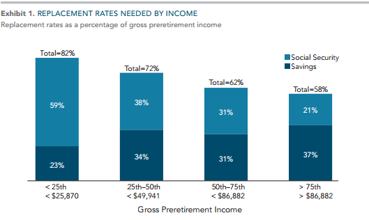
Exhibit 1 shows replacement rates from Lee (2012). As a percentage of gross, preretirement income, replacement rates range from 82% for the bottom 25% of the income distribution to 58% for the top 25%. Low-income households can rely on Social Security to replace most of their preretirement income, while high earners need to rely more on personal savings. For households with no pension income, replacement rates out of personal savings are estimated to be between 23% for the lowest income quartile and 37% for the top quartile. Based on these estimates, we use a conservative 40% replacement rate for our analysis.
STEP 2: CALCULATING A SAVING RATE
Given a replacement rate, required saving rates depend on individual income paths, portfolio returns, and assumed withdrawal rates or annuity pricing at retirement. We assume individuals start saving at age 25 and retire at 66, and simulate real income paths and portfolio returns over the working lives of 100,000 households. We assume savings are invested in global equities and fixed income, following a trend allocation strategy, with equity exposure equal to (120 – Age)%.4 At age 65, we calculate a final portfolio value for each of the 100,000 simulated paths; we convert it into retirement income assuming the price of a $1 real annuity is $20. Finally, we find the saving rates that yield a 40% replacement for 95%, 90%, and 50% of the paths.5
SAFETY IS COSTLY
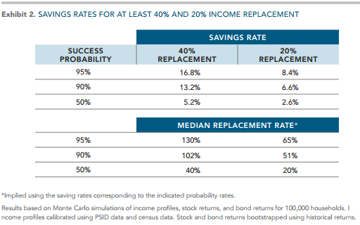
Exhibit 2 shows the saving rates needed for 95%, 90%, and 50% success probabilities. We find that to replace 40% of preretirement income with 95% probability, households need to save 16.8% of their salary from age 25 to 65.6 For a 90% success rate, the savings rate needed is 13.2%, and it is substantially lower for a 50% success rate, which can be achieved with less than a third of the savings needed for 95% probability.
The change in saving rates required to increase the probability of success is a measure of the cost to safeguard against shortfalls using the assumed allocation strategy.
Exhibit 2 shows that safety is costly.
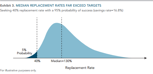
The high saving rates required for a 95% probability of success result in median replacement rates that far exceed the targeted 40%. The median replacement rate is 130% when targeting 40%, as shown in Exhibit 3. Thus, higher saving rates result in a tradeoff between current consumption and higher expected retirement income.7
STARTING EARLY MATTERS
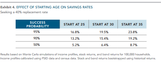
We have so far assumed that individuals start saving at age 25 and save constantly until age 65. What about individuals who start saving later? Exhibit 4 shows saving rates for individuals who begin saving at ages 30 or 35, seeking a 40% replacement. An individual who targets a 90% success rate needs to save 15.4% if he starts at age 30 or 19.2% if he starts at age 35—much higher than the 13.2% saving rate required when starting at age 25. Starting early and saving consistently should be a priority when planning for retirement.
INCOME PATHS MATTER
When planning for retirement, future income paths are largely unknown. Defining a retirement goal as an income replacement rate is a sensible way to manage this uncertainty, because as earnings rise over time, target retirement income increases, as well. But this approach will not work well for everyone. In particular, for individuals in the upper end of the income distribution at 65, for whom income growth is greater than expected, relatively low savings at the beginning of their career will not be enough to replace the high income earned as they neared retirement.
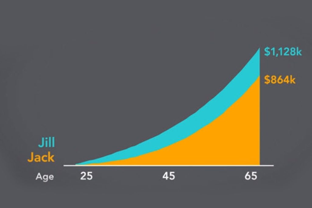
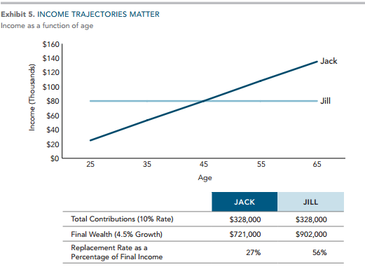
Consider two examples: Jill, with real earnings of $80,000 a year throughout her career; and Jack, starting at 25 with $25,000 per year and ending at age 65 making $135,000. They both make $80,000 a year on average over their employment life, so with the same constant saving rate, they will have the same cumulative contributions (Exhibit 5). But more of Jill’s contributions occur earlier in life, so she will have a larger final balance at 65. With a lower income at 65, she will have a higher replacement rate than Jack. Alternatively, she needs to save less than Jack to achieve the same replacement rate.
By simulating realistic income trajectories, we find that most of the households that fail to meet the target replacement are households with steep income growth.8 Individuals with this income pattern are likely to need higher saving rates than the ones in Exhibit 2. We develop a potential solution in the next section.
INCORPORATING INCOME TO IMPROVE SUCCESS RATES
Not everyone experiences high-income growth. Nor can everyone afford to consistently save large fractions of their income. Young households may find it hard to save the 16.8% required for a 95% success rate. And if they experience high growth (relatively likely among the highly educated), even this rate may not be enough. For young households, current consumption and housing expenses often take priority over retirement savings. For example, results from the 2007 the Survey of Consumer Finances show that only 9% of individuals younger than 25 consider saving for retirement a priority. This percentage increases steadily over the working years and peaks in the late 50s at 59%.9 As a result, individuals are more likely to save relatively more as their age and income increase.
In addition, more is known about one’s income path as time goes by. One way to improve the chances of a successful retirement—particularly for individuals who experience higher income growth—is to have saving rates change as income changes. A natural way to increase the success rate is to increase the rate of saving as income increases.
A saving rule in which the saving rate increases with income is consistent with standard economic theory. Households should strive to smooth consumption over time. Debt and savings are the tools households use to shift consumption from one period to another. Since income is low early in life, life cycle models predict young households will spend the bulk of their earnings. It might even be rational for them to borrow against future income to support more spending early in life. As income grows, households need to shift into savings mode in preparation for retirement. Life cycle theories are generally supported empirically, and academic research shows that saving rates do increase with income.10
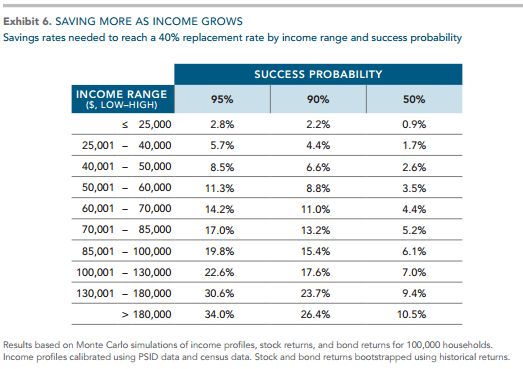
To derive saving rates that increase with income, we first identified 10 income groups of approximately similar sizes. Then we calculated saving rates for each income bucket that increase as income rises. The results are shown in Exhibit 6. A 25-year-old making $48,000 can start by saving 6.6% for a 90% probability of success, and gradually increase savings through time (to 8.8% as he crosses the $50,000 threshold, 11% as he crosses $60,000, etc.). If he has a college degree, his income is expected to peak at $120,000 by age 45. At that time, he should be saving 17.6%. It is intellectually satisfying that saving rates in this table are broadly consistent with the evidence in Dynan, Skinner, and Zeldes (2004). The good news is that saving rates do not need to be as high as in Exhibit 6 throughout one’s working life, but they do need to be high as income increases and when the capacity to save is also higher. In addition, the saving rates in Exhibit 6 result in relatively even success rates across the range of final income.
AM I ON TRACK? EFFECT OF SAVING AND ACCUMULATED ASSETS
Over time, individuals may deviate from their savings plans because of unexpected personal events, higher or lower accumulated assets than expected, or changes in retirement goals. In any event, it is good practice to evaluate one’s progress and make appropriate changes if needed.
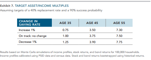
A useful measure of intermediate performance is accumulated assets divided by current income, the assetincome multiple. The greater this multiple is, the greater the chance to achieve a given target replacement rate. Given an asset-income multiple, we can calculate the additional saving (or dissaving) needed to meet a replacement rate going forward. If the asset-income multiple is too low, additional savings are needed (relative to a previously followed rule). If the asset-income multiple is very high, the savings rate could be reduced to target a given success probability.
Exhibit 7 shows target asset-income multiples at intermediate ages 35, 45, and 55, for a 90% success rate. It also shows asset-income levels for which a 1 percentage point adjustment (up or down) in the saving rate is required to be on track. A 35-year-old targeting a 40% replacement with an asset-income multiple of 1.00 is on track and can continue with the rule of Exhibit 7 but would need to increase the saving rate by 1 percentage point with assets equal to 0.75 times his current income. He could decrease the saving rate by 1 percentage point with 1.25 times his current income.
CONCLUSION
Determining how much to save for retirement is challenging, given the high uncertainty about income, portfolio returns, and spending needs many years into the future. Given this uncertainty, and the high heterogeneity of earning potential and spending needs, what works well on average does not work well for everyone. A one-size-fits-all savings rate during one’s working life may be too high for some and too low for others.
Our study tries to provide some general guidelines. First, start early, even at low saving rates. Missed years have a non-trivial impact on future saving rates, and the early buildup of assets can offer flexibility later in life. Similarly, save consistently over time. Increase savings with income, as in Exhibit 5, particularly if you are uncertain about future income growth. This will bring down savings rates for low earners without compromising chances for individuals who will experience high income growth. Third, keep track of performance by monitoring accumulated savings and savings rates as income changes, and make changes as needed—along the lines of Exhibit 5. Consistent with these guidelines, and in the spirit of minimizing the cost of saving, take maximum advantage of employer contributions.
We calculate savings rates based on ideal savings and investment behavior: Saving is consistent, there is no leakage from hardship loans or fees, and investors remain disciplined in their asset allocation. For plan sponsors, our results point to the importance of institutionalizing consistent savings though better plan design. Automaticity is one of the tools plan sponsors can use to help participants start saving for retirement the moment they join the plan. Combined with auto-escalation, a well-designed plan can guide participants to save more over time (again, keeping with standard economic theory, which states savings rates should increase with income). With respect to performance, oversight by fiduciaries offers the greatest opportunity to help guide participants to better outcomes based on fiduciaries’ responsibility to prudently monitor and select participant investment options.i The other side of the “performance coin” is fees; the same fiduciary oversight is needed in order to ensure fees are not only reasonable, but also reasonable in light of the value received.
We hope this primer on savings starts the conversation regarding DC plan design with the ultimate goal of helping participants achieve their desired income replacement rate in retirement.
1. PSID stands for Panel Study on Income Dynamics, directed by faculty at the University of Michigan.
2. Please refer to the white paper version of our study for a more complete treatment of these questions, as well as others.
3. Marlena Lee, “The Retirement Income Equation,” DC Dimensions (Summer 2012). Refer to this paper for a more complete discussion about replacement rates.
4. The portfolios are rebalanced yearly in the simulation. Global equity returns are from the Dimson-Marsh-Staunton Global Returns database. Five-year Treasury notes are from Ibbotson. The data cover the period 1926 to 2011. Real annual equity returns average 7.7%, with a standard deviation of 19%. Real returns on five-year Treasury notes average 2.5%, with a std deviation of 6.8%.
5. As is typical in this type of simulation, we interpret the frequency with which a replacement rate is achieved across paths as an estimate of the probability of success, or success rate.
6. These are total savings rates into personal accounts, so they would include any employer contributions.
7. The cost of this safety, in terms of saving rates, can possibly be reduced by using allocations that give up upside potential. See the white paper version of this study for additional discussion.
8. The data shows a high degree of heterogeneity in income trajectories. We refer to our white paper version of this study for more discussion about income variability and how it is incorporated in our simulations.
9. See Figure 1 in Andrew Samwick, “The Design of Retirement Saving Programs in the Presence of Competing Consumption Needs,” National Tax Association Proceedings (2010).
10. See, for example, K.E. Dynan, J. Skinner, and S. P. Zeldes, “Do the Rich Save More?” Journal of Political Economy 112, no. 2 (2004). For a review of lifecycle theory and empirical evidence, see M. Browning and T. F. Crossley, “The Life-Cycle Model of Consumption and Saving,” Journal of Economic Perspectives 15, no. 3 (2001).
i. ERISA § 404(a)(1)(B).
